Shiny + deSolve = Interactive ODE Models
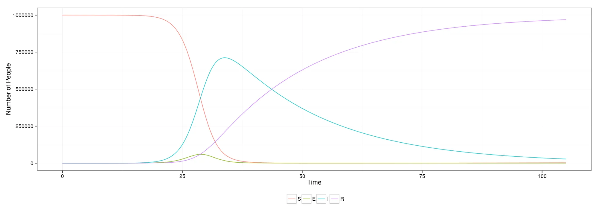
While taking a disease dynamics course, I thought it would be a good opportunity to learn how to use the Shiny package in R and create an interactive interface for some of my problem sets. After a few trial runs with smaller, simpler setups, I have wrapped up the side project (for now). You can see it in action here 1 and you can view the final code on my Git.
At some point, I’d like to make an analogous version of these models using network-based approaches. However, all my work in network models has been done using Python so it might take a while.
If you’re unfamiliar with compartmental models, they are deterministic models that use differential equations to describe the spread of an epidemic through a population. The Wikipedia page on them is a pretty good place to start. The parameters on the page are described below—note that certain parameters are only shown when they are applicable.
- Basics:
- Probability of transmission: the probability that an infectious person will infect a susceptible person at any one contact.
- Average contacts: the number of people an infected person will run into (per week).
- Disease properties:
- No recovery: when checked, if somebody becomes infected, they will be infectious forever—never recovering.
- Duration: how long an infected person remains infected
- Latent period: the time between being infected and being infectious (at which point they are neither susceptible nor infected, but are “exposed”).
- Seasonal fluctuations: a cosine function that emulates seasonal fluctuations in contact rates.
- Vital dynamics:
- Birth and death rate: Self-explanatory. In these model, kept equal to each other.
- Proportion of vaccinated a birth: assumes vaccination occurs immediately at birth (therefore, this is the proportion of new births who never enter a susceptible stage).
- Vaccine effectiveness: probability of a vaccine actually working.
Footnotes
-
Updated 02/13/15 — moved to shinyapps.io ↩